Multi-Product Simulation ¶

Stockpyl supports simulating systems with multiple products. This page describes how to create and manage products, as well as simulate multi-product systems. If you haven’t already read the the tutorial page for simulation, read that first.

Note

The terms “node” and “stage” are used interchangeably in the documentation.

Note

The notation and references (equations, sections, examples, etc.) used below refer to Snyder and Shen, Fundamentals of Supply Chain Theory (FoSCT), 2nd edition (2019).

Products ¶

The primary class for handling products is the SupplyChainProduct. A SupplyChainProduct object is typically added to one or more SupplyChainNode objects; those nodes are then said to “handle” the product. Most attributes (local_holding_cost, stockout_cost, demand_source, inventory_policy, etc.) may be specified either at the node level (same value for all products at the node), at the product level (same value for all nodes that handle the product), or at the node-product level (separate value for the node-product pair).

Products are related to each other via a bill of materials (BOM). The BOM specifies the number of units of an upstream product (raw material) that are required to make one unit of a downstream product (finished goods). For example, the BOM might specify that 5 units of product A and 2 units of product B are required to make 1 unit of product C at a downstream node. The raw materials are products A and B, and the finished good is product C.

Note

“Raw materials” and “finished goods” are SupplyChainProduct objects. They are not separate classes. Moreover, a finished good at one node may be a raw material at another node; for example, node 1 might produce product A as its finished good, which it then ships to node 2, where it is used as a raw material to produce product B.

Dummy Products ¶

Every node has at least one product. If your code does not explicltly create products or add them to nodes, Stockpyl automatically creates and manages “dummy” products at each node. This means that you can ignore products entirely if you do not need them, and you can build and simulate networks just as you did in versions prior to Stockpyl prior to v1.0 (when products where introduced).

When a product is added to a node, the dummy product is removed. If all “real” products are removed, a dummy product is added back.

Dummy products are identifiable as such because they have negative indices, or because their is_dummy attribute is set to True.

Basic Multi-Product Example ¶

This tutorial will use the following network:

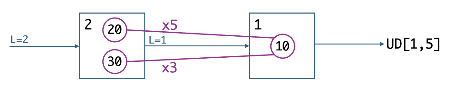
In the diagram:

The squares represent nodes. The number in the top-left corner of a node is its index.

The circles represent products. The number in a product is its index.

The lines from products 20 and 30 to product 10 indicate that products 20 and 30 are raw materials that are used to make product 10. To make 1 unit of product 10 requires 5 units of product 20 and 2 units of product 30, as indicated by x5 and x3 on the lines.

The arrow from node 2 to node 1 indicates that node 2 ships items to node 1. The lead time for these shipments is 1 period, as indicated by L=1 on the arrow.

The arrow from node 1 represents the external demand, which follows a uniform discrete distribution on [1,5].

The arrow into node 2 represents the external supplier. The lead time for shipments from the external supplier is 2 periods, as indicated by L=2 on the arrow.

We’ll start building this network using the serial_system() function:

>>> from stockpyl.supply_chain_network import serial_system
>>> network = serial_system(
...     num_nodes=2,
...     node_order_in_system=[2, 1],
...     node_order_in_lists=[1, 2],
...     stockout_cost=[20, 0],
...     demand_type='UD',
...     lo=1,
...     hi=5,
...     shipment_lead_time=[1, 2]
...     )
>>> # Build a dict for easier access to the nodes.
>>> nodes = {n.index: n for n in network.nodes}

Next, we’ll create the three products and add them to a dict whose keys are product indices and whose values are products, for easy access to the product objects. We’ll also set the BOM.

>>> from stockpyl.supply_chain_product import SupplyChainProduct
>>> products = {10: SupplyChainProduct(index=10), 20: SupplyChainProduct(index=20), 30: SupplyChainProduct(index=30)}
>>> products[10].set_bill_of_materials(raw_material=20, num_needed=5)
>>> products[10].set_bill_of_materials(raw_material=30, num_needed=3)

To add the products to the nodes, we use add_product() and add_products():

>>> nodes[1].add_product(products[10])
>>> nodes[2].add_products([products[20], products[30]])

Assigning Attributes ¶

Most attributes that apply to nodes (local_holding_cost, stockout_cost, demand_source, inventory_policy, etc.) also apply to products. There are three ways to assign attributes:

By setting it at a node, e.g., my_node.stockout_cost = 50

By setting it at a product, e.g., my_product.stockout_cost = 50
By setting the attribute at the node to a dict whose keys are product indices and whose values are the attribute values, e.g.,
my_node.stockout_cost = {my_product1.index: 50, my_product2.index: 70}
This allows you to set (node, product)-specific values of the attribute

In our example network, since node 1 only handles one product (product 10), we can set local_holding_cost directly at node 1. We’ll set local_holding_cost for products 20 and 30 in the product objects.

>>> nodes[1].local_holding_cost = 5
>>> products[20].local_holding_cost = 2
>>> products[30].local_holding_cost = 3

We need an inventory policy for each product. This attribute, too, can be set at the node, product, or (node, product) levels. We’ll set the policy for product 10 in the product object (we could instead set it at node 1). And we’ll set the policy for products 20 and 30 using a dict at node 2:

>>> from stockpyl.policy import Policy
>>> products[10].inventory_policy = Policy(type='BS', base_stock_level=6, node=nodes[1], product=products[10])
>>> nodes[2].inventory_policy = {
...     20: Policy(type='BS', base_stock_level=35, node=nodes[2], product=products[20]),
...     30: Policy(type='BS', base_stock_level=20, node=nodes[2], product=products[30])
... }

Accessing Attributes ¶

It is possible to access attributes in the same way they were assigned:

>>> nodes[1].local_holding_cost
5
>>> products[20].local_holding_cost
2
>>> products[30].local_holding_cost
3
>>> products[10].inventory_policy
Policy(BS: base_stock_level=6.00)
>>> nodes[2].inventory_policy[20]
Policy(BS: base_stock_level=35.00)

But it can be annoying to access them this way, because you need to know whether the attribute was originally assigned to the node, to the product, or to the node as a dict.

Instead, use the get_attribute() method, which figures out where the attribute is set and returns the appropriate value. In particular, the method attempts to access the attribute in the following order:

As a dict in the node object (meaning there is a (node, product)-specific value)

As a singleton in the product object (meaning there is a product-specific value)

As a singleton in the node object (meaning there is a node-specific value)

(If none of these, an exception is raised)

During a simulation, Stockpyl uses get_attribute() to access all attributes, so the simulation will pull attributes from nodes and products using the same logic as above.

>>> nodes[1].get_attribute('local_holding_cost', product=10)
5
>>> nodes[2].get_attribute('local_holding_cost', product=20)
2
>>> nodes[2].get_attribute('local_holding_cost', product=30)
3
>>> # You can omit the `product` argument if the node has a single product.
>>> nodes[1].get_attribute('inventory_policy')
Policy(BS: base_stock_level=6.00)
>>> nodes[2].get_attribute('inventory_policy', product=20)
Policy(BS: base_stock_level=35.00)

Bill of Materials ¶

The number of units of product A required to make 1 unit of product B is called the BOM number for products A and B. The BOM number is specified at the product level, not the node level: If the BOM number for products A and B is 5, then it is 5 no matter what nodes are under consideration.

The set_bill_of_materials() method is used to set the BOM relationships between pairs of products. We already used the following code to set the BOM for our example network:

>>> products[10].set_bill_of_materials(raw_material=20, num_needed=5)
>>> products[10].set_bill_of_materials(raw_material=30, num_needed=3)

We can access the BOM number using get_bill_of_materials(), or the shortcut method BOM():

>>> products[10].get_bill_of_materials(raw_material=20)
5
>>> products[10].BOM(30)
3

In a Stockpyl simulation, every network must have external supply—nodes can’t just create a product with no raw materials. (See External Suppliers.) To specify that a node receives external supply, you set that node’s supply_type attribute to 'U' (for “unlimited”), or to anything other than None. The serial_system() function automatically sets supply_type = 'U' for the upstream-most node, which means that node 2 in our network has external supply.

External suppliers provide raw materials, even though they are not created explictly as SupplyChainProduct objects. The BOM for such raw materials is therefore also not specified explicitly. Instead, such relationships are governed by the network bill of materials (NBOM), which assigns default values to certain pairs of nodes/products based on the structure of the network. The basic rule is:

Network Bill of Materials (NBOM)

If node A is a predecessor to node B, and there are no BOM relationships specified between any product at node A and any product at node B, then every product at node B is assumed to require 1 unit of every product at node A as a raw material.

In the case of our example network, that means that product 20 and product 30 require 1 unit of the product provided by the external supplier. (That item is a “dummy” product assigned to the supplier.)

We don’t set the NBOM explicitly—we only set the BOM, and Stockpyl automatically adds the network-based relationships as needed. We can query the NBOM using get_network_bill_of_materials() (or its shortcut, NBOM()), which returns the BOM relationship for a given (node, product) and a given (predecessor, raw material). If the BOM is set explicitly, get_network_bill_of_materials() returns that number, and if it’s implicit from the network structure, it returns that number. If there is no BOM relationship (either explicit or implied), it returns 0.

If an NBOM relationship is implied by the network structure, the NBOM always equals 1. If you want it to equal something else (e.g., if we wanted to say that 4 units of the external supplier product are required to make 1 unit of product 30), you would need to explicitly create a node that’s a predecessor to node 2, create a product at that node that’s a raw material for product 30, and set the BOM explicitly.

>>> # Get the NBOM for node 1, product 10 with node 2, product 20.
>>> nodes[1].NBOM(product=10, predecessor=2, raw_material=20)
5
>>> # Get the NBOM for node 2, product 20 with the external supplier's dummy product.
>>> nodes[2].NBOM(product=20, predecessor=None, raw_material=None)
1

Raw Material Inventory ¶

Every node has a raw material inventory for every product that it uses as a raw material. So, in our example, node 1 has raw material inventory for products 20 and 30, and node 2 has raw material inventory for the dummy product from the external supplier. The holding cost rate for raw material inventory is the same as the holding cost for the same product at the node that supplies it. (This node is chosen arbitrarily if there are multiple such nodes.)

Raw material inventories are by product only, not by (product, predecessor). There are two important implications of this:

If a node has multiple suppliers that provide the same raw material, those supplies are pooled into a single raw material inventory.

If a node has multiple products that use the same raw material, they share the same raw material inventory.

The second bullet is relevant for our example network, because both product 20 and product 30 use the dummy product from the external supplier as a raw material, so they both draw their raw materials from the same inventory.

Multi-Product Simulation Output ¶

This section discusses the simulation output for a multi-product network, i.e., a network in which one or more SupplyChainProduct objects have been added explicitly. (See Simulation Output for an overview of the sim_io module and the simulation output in the context of a single-product network.)

The write_results() function displays the results of the simulation in a table. The table has the following format for multi-product networks:

Each row corresponds to a period in the simulation.

Each node is represented by a group of columns.

The node number is indicated in the first column in the group (i.e., i=1).

(node, product) pairs are indicated by a vertical line, so ‘2|20’ means node 2, product 20.

The columns for each node are as follows:

i=<node index>: label for the column group

DISR: was the node disrupted in the period? (True/False)

IO:s|prod: inbound order for product prod received from successor s

IOPL:s|prod: inbound order pipeline for product prod from successor s: a list of order quantities arriving from succesor s in r periods from the period, for r = 1, …, order_lead_time

OQ:p|rm: order quantity placed to predecessor p for raw material rm

OQFG:prod: order quantity of finished good prod (this “order” is never actually placed—only the raw material orders in OQ are placed; but OQFG can be useful for debugging)

OO:p:rm: on-order quantity (items of raw material rm that have been ordered from successor p but not yet received)

IS:p|rm: inbound shipment of raw material rm received from predecessor p

ISPL:p|rm: inbound shipment pipeline for raw material rm from predecessor p: a list of shipment quantities arriving from predecessor p in r periods from the period, for r = 1, …, shipment_lead_time

IDI:p|rm: inbound disrupted items: number of items of raw material rm from predecessor p that cannot be received due to a type-RP disruption at the node

RM:rm: number of items of raw material rm in raw-material inventory at node

PFG:prod: number of items of product prod that are pending, waiting to be processed from raw materials

OS:s|prod: outbound shipment of product prod to successor s

DMFS|prod: demand of product prod met from stock at the node in the current period

FR|prod: fill rate of product prod; cumulative from start of simulation to the current period

IL|prod: inventory level of product prod (positive, negative, or zero) at node

BO:s|prod: backorders of product prod owed to successor s

ODI:s|prod: outbound disrupted items of product prod: number of items held for successor s due to a type-SP disruption at s

HC: holding cost incurred at the node in the period

SC: stockout cost incurred at the node in the period

ITHC: in-transit holding cost incurred for items in transit to all successors of the node

REV: revenue (Note: not currently supported)

TC: total cost incurred at the node (holding, stockout, and in-transit holding)

For state variables that are indexed by successor, if s = EXT, the column refers to the node’s external customer

For state variables that are indexed by predecessor, if p = EXT, the column refers to the node’s external supplier

Negative product indices are “dummy products”

Example: The code below simulates our example network for 10 periods and displays the results. It sets the rand_seed parameter to allow the results to be reproduced.

>>> simulation(network=network, num_periods=10, rand_seed=17)
>>> write_results(network, num_periods=10, columns_to_print=['basic', 'costs', 'RM', 'ITHC'])

The results are shown in the table below. In period 0:

We start with IL:10 = 6 at node 1, IL:20 = 35 and IL:30 = 20 at node 2. (By default, the initial inventory level equals the base-stock level.) These numbers aren’t displayed in the table below, only the ending ILs are.

Node 1 receives a demand of 2 for product 10 (IO:EXT|10 = 2). Its inventory position (IP) is now 6 - 2 = 4 and its base-stock level is 6, so it needs to order 2 units’ worth of raw materials. Expressed in the units of the raw materials, that means it needs to order 10 units of product 20 (because BOM = 5) and 6 of product 30 (because BOM = 3). In the table, OQ:2|20 = 10, OQ:2|30 = 6.

Node 1 has sufficient inventory to fulfill the demand of 2, so it does (OS:EXT|10 = 2).

Node 1 ends the period with IL:10 = 4, and incurs a holding cost of 20 since the per-unit holding cost is 5. There is no stockout cost in this period, so we have HC = 20, SC = 0, TC = 20.

Node 2 receives an inbound order of 10 units for product 20 and 6 units for product 3 (IO:1|20 = 10, IO:1|30 = 6). Its inventory positions are now IP:20 = 35 - 10 = 25, IP:30 = 20 - 6 = 14 and its base-stock levels are 35 and 20, respectively. So it needs to order 10 units of the raw material from the external supplier for product 20, and another 6 units of raw material for product 30. (Remember that the NBOM = 1 for these pairs.) So, OQ:EXT|-5 = 16. (-5 is the index of the dummy product at the external supplier.) Of those 16 units, 6 are “earmarked” for product 20 and 10 are for product 30.

Node 2 has sufficient inventory to satisfy demand for both products, so it ships 10 units of product 20 and 6 units of product 30 (OS:1|20 = 10, OS:1|30 = 6).

Node 2 ends the period with IL:20 = 25, IL:30 = 14, so HC = 25 * 2 + 14 * 3 = 92 and SC = 0. Node 2 also incurs the in-transit holding cost for items that it shipped to node 1 that have not arrived yet; there are 10 units of product 20 and 6 units of product 30, and the holding cost rates are 2 and 3, so ITHC = 10 * 2 + 6 * 3 = 38; and TC = 92 + 38 = 130.

In period 1:

Node 1 starts period 1 with an IL of 4, and has 10 units of product 20 and 6 units of product 30 on order (OO:2|20 = 10 and OO:2|30 = 10 at the end of period 0). The on-order units are sufficient to produce 2 units of product 10, so its starting IP is 4 + 2 = 6.

Node 1 receives a demand of 2 again (IO:EXT|10 = 2), so its new IP is 4, and it again orders 10 units of product 20 and 6 of product 30 (OQ:2|20 = 10, OQ:2|30 = 6).

Node 1 again meets the demand in full (OS:EXT|10 = 2), ends the period with IL:10 = 4, and has costs HC = 20, SC = 0, and TC = 20.

Node 2 starts period 1 with IL:20 = 25. It has 16 units of its raw material on order from the external supplier (OO:EXT|-5 = 16 at the end of period 0), 10 of which were “earmarked” for product 20, so its starting IP for product 20 is 25 + 10 = 35. Node 1 ordered 10 units of product 20, so its new IP is 35 - 10 = 25. Its base-stock level for product 20 is 35, so it will need to order 10 units of the raw material from the external supplier for product 20.

For product 30, the starting IL is 14, the on-order inventory is 10 (of which 6 were “earmarked” for product 30), the demand is 6, so the IP is 14 + 6 - 6 = 14. The base-stock level for product 30 is 20, so the node needs to order 6 units of the raw material. Therefore, node 2 places an order for a total of 16 units of the raw material from the external supplier (OQ:EXT|-5 = 16).

Node 2 again has sufficient inventory to meet its full demand, so OS:1|20 = 10 and OS:1|30 = 6.

Node 2 ends period 1 with IL:20 = 25 - 10 = 15 and IL:30 = 14 - 6 = 8, so HC = 15 * 2 + 8 * 3 = 54. There are 10 units of product 20 and 6 of product 30 in transit to node 1, so ITHC = 10 * 2 + 6 * 3 = 38; and TC = 54 + 38 = 92.

Here’s an explanation of the fractional order quantities at node 1 in period 5:

Node 1 starts period 5 (ends period 4) with 1 unit of the finished good, product 10 (IL:10 = 1 in period 4), and 0 units of both product 20 and product 30 in raw material inventory (RM:20 = 0, RM:30 = 0 in period 4).

Node 1 receives 10 units of product 20 and 5 of product 30 in period 5 (IS:2|20 = 10, IS:2|30 = 5).

Now node 1 has 10 units of product 20 and 5 of product 30 on hand, which is enough to make 1.6667 units of product 10 at node 1. Doing so uses up all units of product 30 and 5 * 1.6667 = 8.3333 units of product 20, leaving 1.6667 remaining units of product 20.

Therefore, node 1 ends period 5 with RM:20 = 1.6667 and RM:30 = 0.

The demand for product 10 in period 5 is 5 (IO:EXT|10 = 5). Node 1 began the period with 1 unit of product 10 and then producted 1.6667 additional units; it ships these 2.6667 units to the external customer (OS:EXT|10 = 2.6667) and ends the period with 2.3333 backorders (IL:10 = -2.3333). It incurs a holding cost on the raw material inventory of product 20, at the per-unit local holding cost rate for product 20, i.e., 2. So HC = 2 * 1.6667 = 3.3333. It incurs a stockout cost of 20 per backorder, so SC = 20 * 2.3333 = 46.6667, and TC = 3.3333 + 46.6667 = 50.

Multi-Product Simulation Results¶
t	IO:EXT\|10	OQ:2\|20	OQ:2\|30	OO:2\|20	OO:2\|30	IS:2\|20	IS:2\|30	RM:20	OS:EXT\|10	IL:10	HC	SC	TC	IO:1\|20	IO:1\|30	OQ:EXT\|-5	OO:EXT\|-5	IS:EXT\|-5	OS:1\|20	OS:1\|30	IL:20	IL:30	HC	ITHC	TC
0	2	10	6	10	6	0	0	0	2	4	20	0	20	10	6	16	16	0	10	6	25	14	92	38	130
1	2	10	6	10	6	10	6	0	2	4	20	0	20	10	6	16	32	0	10	6	15	8	54	38	92
2	1	5	3	5	3	10	6	0	1	5	25	0	25	5	3	8	24	16	5	3	20	11	73	19	92
3	5	25	15	25	15	5	3	0	5	1	5	0	5	25	15	40	48	16	25	15	5	2	16	95	111
4	5	25	15	25	15	25	15	0	5	1	5	0	5	25	15	40	80	8	10	5	-15	-10	0	35	35
5	5	25	15	40	25	10	5	1.6667	2.6667	-2.3333	3.3333	46.6667	50	25	15	40	80	40	25	15	-15	-10	0	95	95
6	2	10	6	25	16	25	15	1.6667	4.3333	0.6667	6.6667	0	6.6667	10	6	16	56	40	25	15	0	-1	0	95	95
7	2	10	6	10	7	25	15	1.6667	2	3.6667	21.6667	0	21.6667	10	6	16	32	40	10	7	15	8	54	41	95
8	2	10	6	10	6	10	7	0	2	4	20	0	20	10	6	16	32	16	10	6	15	8	54	38	92
9	1	5	3	5	3	10	6	0	1	5	25	0	25	5	3	8	24	16	5	3	20	11	73	19	92

Download table in CSV format

Accessing the State Variables ¶

In addition to viewing the results in tabular form, you can also query a NodeStateVars object to get values of individual state variables, using methods such as get_inventory_level(), get_order_quantity(), etc. The arguments of these methods are the relevant nodes/products, but these arguments can be omitted if they are inferrable (e.g., if the node has a single predecessor, or a single product, etc.).